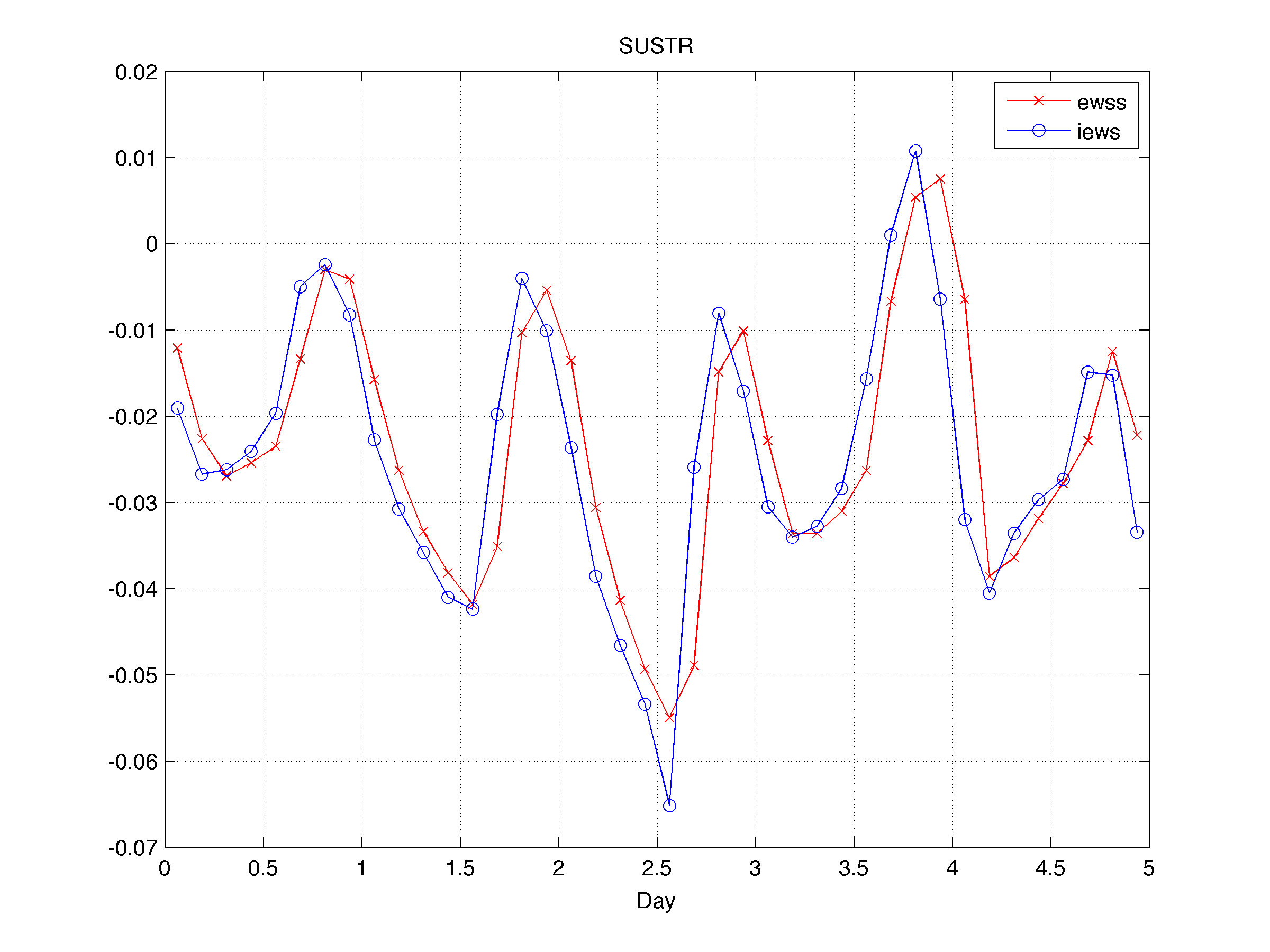
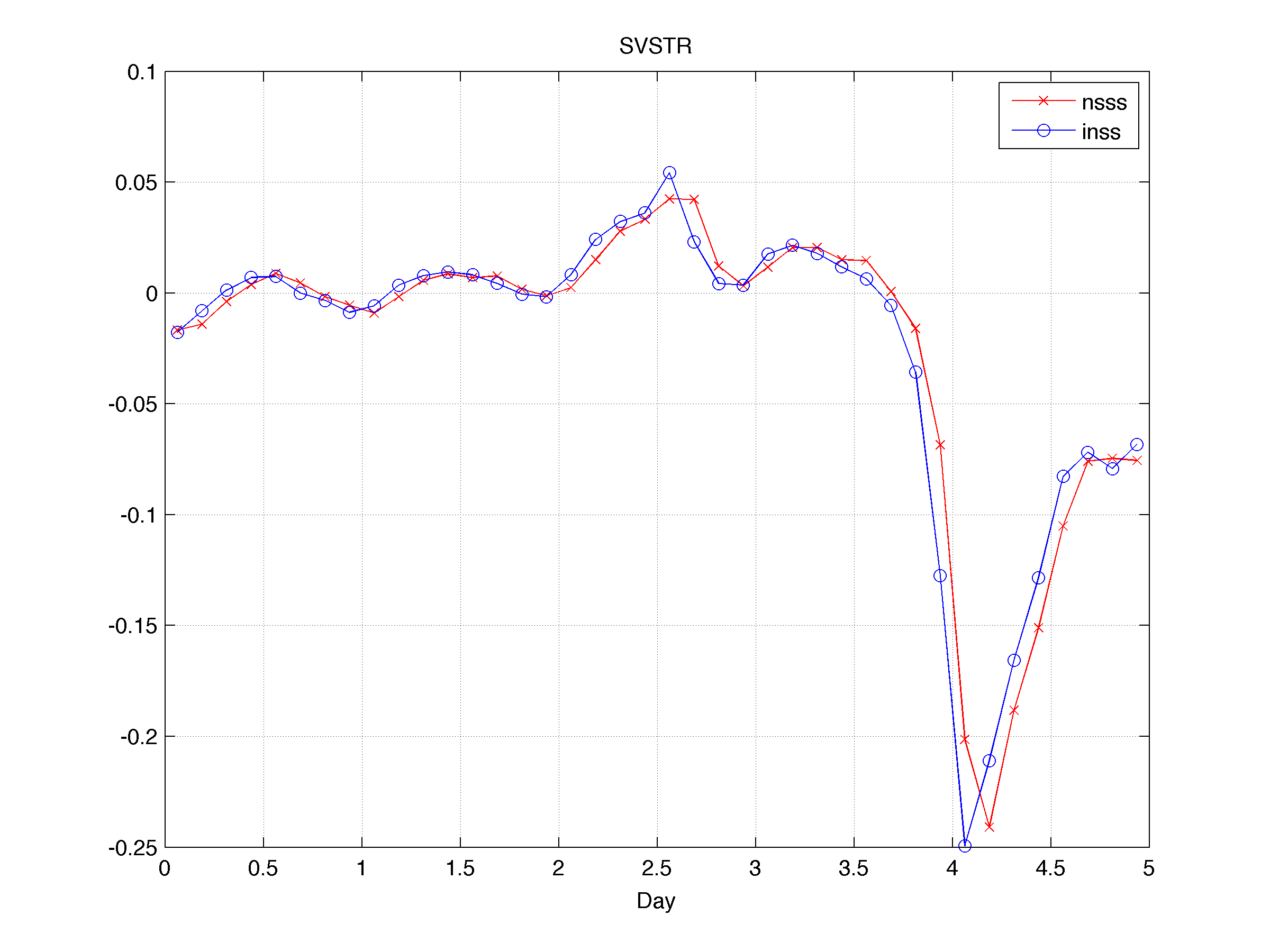
The explanation is kind of complicated. The bulk flux formulation in ROMS uses the Monin-Obukhov similarity parameters of Liu et al. (1979) to compute stability functions that compute the turbulent fluxes for wind (Wstar), heat (Tstar), and moisture (Qstar). There are stable and unstable regimes for these functions. This computation can be highly nonlinear. Any bias or errors in the open boundary conditions for temperature, due to radiation conditions, may result in a loss or gain of heat at the boundary. This may create bogus upwelling/downwelling at the open boundary edges. The model becomes unstable quite rapidly and it blows up.
Therefore, I avoid to use BULK_FLUXES in applications with dynamically active circulation regimes. I get instead the total net heat flux and wind stress from a dataset or interpolate them from the coarse model. I usually use the fluxes from
I usually get the following variables from the ERA dataset: The @ denotes accumulated quantity that must be divided by the time interval into the cycle 3, 6, 9 or 12 hours:
Code: Select all
 Select time:   00:00:00     12:00:00
 Select step:   0  3  6  9  12

 @  sshf    W m-2 s        surface sensible heat flux
 @  slhf    W m-2 s        surface latent heat flux
 @  ssr     W m-2 s        surface net solar radiation (shortwave)
 @  str     W m-2 s        surface net thermal radiation (longwave)
 @  strd    W m-2 s        surface thermal radiation downwards
 @  ewss    N m-2 s        east-west surface stress
 @  nsss    N m-2 s        north-south surface stress
 @  e       m              evaporation (downward flux is positive)
 @  ro      m              runoff
 @  tcc     nondimensional total cloud cover [0:1]
 @  tp      m              total precipitation
 @  par     W m-2 s        photosynthetically active radiation at surface
    msl     Pa             mean sea level pressure
    v10v    m s-1          10 metre U wind component
    vl0u    m s-1          10 metre V wind component
    v2t     K              2 metre temperature
    v2d     K              2 metre dewpoint temperature

  This dataset is written in compact way (short numbers). We need to convert to floating-point data and scale to ROMS units:

    Uwind       (m s-1)         v10u
    Vwind       (m s-1)         v10v
    sustr       (N m-2)         ewss / (3*3600);   3-hour step
    svstr       (N m-2)         nsss / (3*3600);   3-hour step
    shflux      (W m-2)         (ssr+str+sshf+slhf) / (3*3000);   3-hour step
    swrad       (W m-2)         ssr  / (3*3600);   3-hour step
    lwrad_down  (W m-2)         strd / (3*3600);   3-hour step
    latent      (W m-2)         slhf / (3*3600);   3-hour step
    sensible    (W m-2)         sshf / (3*3600):   3-hour step
    rain        (kg m-2 s-1)    tp * Rho_w / (3*3600)
    evaporation (kg m-2 s-1)    e  * Rho_w / (3*3600)
    swflux      (cm day-1)      (-e - tp) * 100 / (3/24);  0.125 day step
    cloud       (nondimesional) tcc
    Pair        (mb)            msl / 100;   (1 mb = 100 Pa)
    Tair        (Celsius)       t2m - 273.15;   (1 C = 273.15 K)
    Qair        (percentage)    100 * (E/Es)

  where

    Rho_w = 1000 kg m-3  (water density)

    E  = 6.11 * 10.0 ^ (7.5 * v2d / (237.7 + v2d))    vapor pressure (mb)
                                                      v2d in Celsius

    Es = 6.11 * 10.0 ^ (7.5 * v2t / (237.7 + v2t))    saturation vapor
                                                      pressure (mb)
                                                      v2t in Celsius
Code: Select all
   A3  = V3 / (3*3600)
   A6  = (V6 - V3) / (3*3600)
   A9  = (V9 - V6) / (3*3600)
   A12 = (V12 - V9) / (3*3600)


Notice that I usually get the variables for BULK_FLUXES in case that I want to compare solutions with or without it. If we are not using BULK_FLUXES, ROMS just needs shflux, swflux, swrad (with some CPP options), sustr, and svstr.
I added the Matlab script template forcing/d_ecmwf2roms.m to the matlab repository to guide you how to process these forcing fields.