Initial history file and time stepping

Report or discuss software problems and other woes

Moderators: arango, robertson

Post Reply
Message
Author
austinctodd

Initial history file and time stepping

#1 Unread post by austinctodd »

I've been running some test cases using various advection schemes and HPG algorithms for the flat isopycnal case, in order to estimate the magnitude of spurious currents after smoothing my topography to satisfy the rx1/rx0 conditions. However, I have come across an interesting error in my temperature distribution in the initial output history file.

What I find is that, when plotting a cross-section of the temperature contours from the first history file (his_0001.nc), my isopycnals are not flat. Looking at the code, it appeared that the initial history file should be exactly the initial condition. However, upon plotting a comparison of the the two, this is not the case:
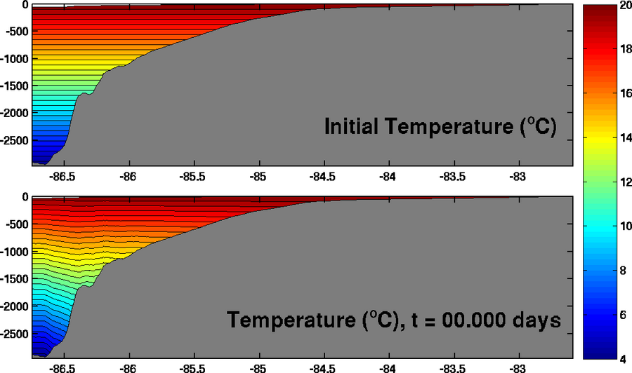
Image

It looks like the model computes some diagnostics, such as KE, PE, volume, etc., but I didn't seem clear to me if any of the initial 3d fields are updated before the first output (esp. since KE is zero):

Code: Select all

   STEP   Day HH:MM:SS  KINETIC_ENRG   POTEN_ENRG    TOTAL_ENRG    NET_VOLUME

      0     0 00:00:00  0.000000E+00  2.810623E+03  2.810623E+03  1.151972E+13
      DEF_HIS   - creating history file: his_0001.nc
      WRT_HIS   - wrote history  fields (Index=1,1) into time record = 0001
If this is the case, then I must have a problem with the reading in of the initial fields. However, I feel like I must be missing something, especially since the spurious mixing appears to be along-slope near the steeper slope. Any suggestions?

User avatar
arango
Site Admin
Posts: 1367
Joined: Wed Feb 26, 2003 4:41 pm
Location: DMCS, Rutgers University
Contact:

Re: Initial history file and time stepping

#2 Unread post by arango »

Hmm, maybe the problem is not in the temperature but in the computation of the depths at RHO-points, which are used to plot the cross-section. How do you compute those depths for each panel in the plot? It looks like the top panel has flat levels and the bottom panel has terrain-following levels, which may locate the same value of temperature at different location in the vertical. Recall that in ROMS the vertical levels are a function of local depth and they evolve in time according to changes in the free-surface.

What are the values of the free-surface in the top and bottom panel? Are you using the correct and official script to compute the ROMS level depths in Matlab. They are distributed in the Matlab repository, see script set_depth.m.

austinctodd

Re: Initial history file and time stepping

#3 Unread post by austinctodd »

I double-checked the calculation of RHO-point depths. It turns out I was using an antiquated piece of code, and they were not exactly the same for the initial interpolation of a linear stratification to my ROMS grid. :oops:

So, upon re-interpolating using the correct depths of RHO points, using the set_depth.m routine, and re-running the model... I find that I arrive at the same problem, even when the initial temperature field actually does have flat isopycnals (on the CORRECT RHO depths!). However, the only place where the isopycnals are not flat occurs at the boundary.

That is, looking one gridpoint away from both the Southern and Western boundary cells, I find flat isopycnals (isotherms):

Image


However, when looking at the boundary grid cell, I do not have flat isopycnals (or isotherms):


Image


Clearly, this is going to generate some currents along the boundary. I am specifying closed boundary conditions, with

Code: Select all

 EASTERN_WALL        Wall boundary at Eastern edge.
 WESTERN_WALL        Wall boundary at Western edge.
 SOUTHERN_WALL       Wall boundary at Southern edge.
 NORTHERN_WALL       Wall boundary at Northern edge.
Again, I didn't think that ROMS changed any of the fields before outputting the initial history file, but perhaps I am overlooking something.

User avatar
arango
Site Admin
Posts: 1367
Joined: Wed Feb 26, 2003 4:41 pm
Location: DMCS, Rutgers University
Contact:

Re: Initial history file and time stepping

#4 Unread post by arango »

OK, that makes sense. ROMS applies boundary conditions to the initial conditions before running the model, see ini_fields.F. This is done for consistency with any of the adjoint-based algorithms. Recall that actually ROMS solves the primitive equation at the interior points and then applies boundary conditions. That is, it is an initial value problem with separate boundary conditions. Nobody applies boundary conditions to the interpolated initial conditions. There are many choices of boundary conditions. In your case, a no gradient boundary conditions is applied.

I will not loose sleep on this one. It is a matter of interpretation between initial and boundary conditions.

austinctodd

Re: Initial history file and time stepping

#5 Unread post by austinctodd »

Ah, yes. I suppose the boundary cell should be zero anyways, because closed boundary conditions would imply that I should be masking those values at the boundary (which I was not doing previously). Adding a masking of those points along the boundary does, in fact zero them out, and allows isopycnals to remain flat one grid cell into the domain.

Thanks for the guidance.

Post Reply